Introduction
This post continues our exploration of insights gained from a year of work with Large Language Models (LLMs). In our previous posts, we discussed general process insights and model-specific observations. Now, we turn our attention to the nuts and bolts of how to actually build LLM-powered applications.
The rapid evolution of LLM capabilities has opened up exciting possibilities for innovation across various industries, including law and business. However, translating these possibilities into practical, efficient, and robust applications is difficult. It feels a bit like the early web. We are always fighting the last war – our tools are optimised for web 2.0 or 3.0 but we’re dealing with web 4.0. There are no textbooks. Everyone is iterating in parallel and capabilities of the models are maturing at a similar rate to the tool being built to help speed up development. There are though some technologies that have adapted well to the new world of LLM API calls.
In this post, we’ll explore several key areas of technical implementation:
- Introduction
- Constructing a Robust Tech Stack for LLM-Powered Systems
- Using Asynchronous Programming
- Parallelisation for High-Quality Output Generation
- Leveraging LLMs in the Development Process
- Prompt Tips
- Conclusion
Constructing a Robust Tech Stack for LLM-Powered Systems
When it comes to building LLM-powered applications, your choice of tech stack can make the difference between a smooth-running system and a nightmarish tangle of spaghetti code. After a year of trial and error, here’s what I’ve found works well – at least for now.
Local or Web-Based Models?
As discussed before, there really is no competition here. The web-based LLMs are far superior to locally hosted versions, despite the reservations on privacy and the need for web-connectivity. You need a hefty processor machine with a large GPU (24GB+) to host a mid-tier novel (similar to the discussed “mini” model capabilities), and that will typically run slower or about the same as a web-based API call.
Backend / Frontend Split
Like many web developers, I’ve come to structure projects with a backend/frontend split. The backend is Python and implements calls to the LLMs. It supplies data in a structured format. The frontend makes it all look pretty and deals with the user interactions. You can build the frontend with Python, but Javascript-based frameworks are more common in production.
Splitting between backend and frontend means that you can later scale these separately. Backend engineers don’t need to worry as much about user interface design and frontend engineers don’t need to worry about complex processing and LLM-wrangling. You can also more easily outsource frontend design to outside agencies, if you have a well-defined backend that does the clever stuff.
Backend: FastAPI with Async Capabilities
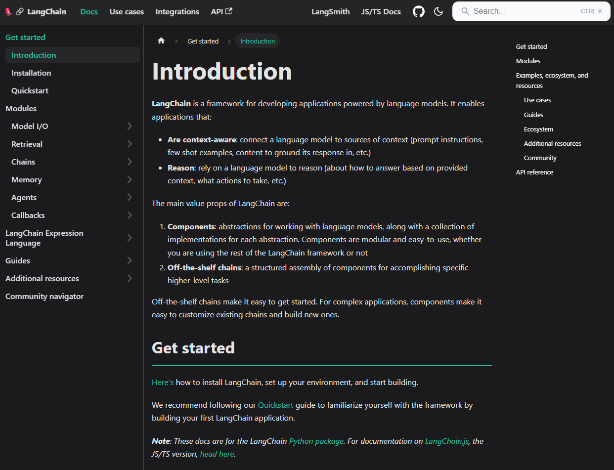
FastAPI has emerged as a go-to framework for building a web API to support LLM applications. It’s fast (as the name suggests), it’s simple, it’s built with async in mind, and it has excellent documentation.
Being the defacto industry standard means there is good support within LLMs and the web for guidance and advice.
The async capabilities are particularly useful when working with LLMs, as we’ll discuss in more detail later.
from fastapi import FastAPI

app = FastAPI()

@app.get("/")
async def root():
    return {"message": "Hello, LLM World"}
Data Validation and API I/O: Pydantic
If you use FastAPI, you’ll be familiar with the use of Pydantic to define the input/output JSON structures of the API. Pydantic is a godsend when it comes to data validation and serialization. It integrates seamlessly with FastAPI and helps catch a multitude of sins before they propagate through your system.
from pydantic import BaseModel

class LLMRequest(BaseModel):
    prompt: str
    max_tokens: int = 100

@app.post("/generate")
async def generate_text(request: LLMRequest):
    # Your LLM logic here
    pass
Using data classes as structures to move data around interfaces is also coming to be used within non-web-facing code as well. This can help when dealing with database objects, where you need to convert database-based classes that require a session object into serialised versions that can be cached and passed between different microservices.
Database Interactions: SQLAlchemy or SQLModel
For database interactions, SQLAlchemy has been the standard for years. However, SQLModel, which builds on SQLAlchemy and Pydantic, is worth keeping an eye on. It’s still maturing, but it offers a more intuitive API for those already familiar with Pydantic.
from sqlmodel import SQLModel, Field

class User(SQLModel, table=True):
    id: int = Field(default=None, primary_key=True)
    name: str
    email: str
I’ve found that SQLAlchemy has a more mature set of documentation for async database access (for SQLAlchemy 2.0). SQLModel’s async documentation is a “Still to Come” holding page. Async database patterns are still a little patchy in terms of support and documentation – definitely not “mature”, more on the “experimental” side of things.
Watch Out
One problem I found is that lots of documentation, tutorials, and examples that feature FastAPI, SQLAlchemy/SQLModel and Pydantic assume a simple non-async use case where all your processing can be performed in your FastAPI route methods. This doesn’t work for LLM applications – if you are fetching anything from an LLM via a web-API (e.g., via the OpenAI or Anthropic Python clients), it will take too long for synchronous web handling – FastAPI is designed to return data quickly from a database in < 200ms, but LLM API calls can often take seconds to complete.
Also many materials only give you solutions that use the syntax for SQLAlchemy 1.x or Pydantic 1.x, which have now been supplanted with 2.x versions.
Application Structure: OOP and Separation of Concerns
When structuring your application, it’s beneficial to separate your business logic from your LLM interaction logic. This makes your code more maintainable and easier to test. Here’s a basic structure I’ve found useful:
my_llm_app/
├── api/
│   ├── routes/
│   └── models/
├── core/
│   ├── config.py
│   └── dependencies.py
├── services/
│   ├── llm_service.py
│   └── business_logic_service.py
├── utils/
└── main.py
As code grows in complexity, there is a need to balance separation of concerns with practical organisation. Real-world projects often have more complex structures than simple examples suggest. Here’s a more comprehensive approach based on actual project structures:
your_project/
├── api/
│   ├── crud/
│   ├── routes/
│   ├── schemas/
│   └── main.py
├── config/
│   ├── __init__.py
│   ├── settings.py
│   └── logging.py
├── database/
│   ├── __init__.py
│   └── db_engine.py
├── logic/
│   ├── chat_processor/
│   ├── database_manager/
│   └── vector_processor/
├── llm/
│   ├── __init__.py
│   ├── embeddings.py
│   ├── prompt_builder.py
│   └── chat_completion.py
├── models/
│   ├── graph/
│   ├── knowledge/
│   └── common.py
├── utils/
├── tests/
│   ├── fixtures/
│   ├── unit/
│   └── integration/
├── migrations/
├── notebooks/
├── docker/
│   ├── Dockerfile.dev
│   ├── Dockerfile.prod
│   └── docker-compose.yml
└── .env
Key aspects of this structure:
- API Layer: Separates routing, CRUD operations, and schema definitions.
- Config: Centralises configuration management, including environment-specific settings.
- Database: Houses database-related code, including code to setup the database and get a session object.
- Logic: Core business logic is divided into focused modules (e.g., chat processing, database management).
- LLM Integration: A dedicated directory for LLM-related functionality, keeping it separate from other business logic.
- Models: Defines data structures used throughout the application.
- Utils: For shared utility functions.
- Tests: Organised by test type (unit, integration) with a separate fixtures directory.
- Docker: Keeps all Docker-related files in one place.
This structure promotes:
- Modularity: Each directory has a clear purpose, making it easier to locate and maintain code.
- Scalability: New features can be added by creating new modules in the appropriate directories.
- Separation of Concerns: LLM logic, business logic, and API handling are kept separate.
- Testability: The structure facilitates comprehensive testing strategies.
Remember, this structure is flexible. Depending on your project’s needs, you might:
- Add a
services/directory for external service integrations. - Include a
frontend/directory for UI components if it’s a full-stack application. - Create a
scripts/directory for maintenance or data processing scripts.
The key is to organise your code in a way that makes sense for your specific project and team. Start with a structure like this, but be prepared to adapt as your project evolves.
Frontend Options
For the frontend, your choice largely depends on your specific needs:
- React: Great for complex, interactive UIs
- Streamlit: Excellent for quick prototyping and data-focused applications
- HTMX: A lightweight option if you want to stick with Python on the frontend
Personally, I’ve found Streamlit to be a lifesaver for rapid prototyping, while React offers the flexibility needed for more complex applications.
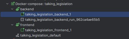
The Glue: Docker and Docker Compose
Finally, Docker and Docker Compose have been invaluable for ensuring consistency across development and production environments. They also make it easier to manage the various components of your stack.
version: '3'
services:
  web:
    build: .
    ports:
      - "8000:8000"
  db:
    image: postgres:13
    environment:
      POSTGRES_DB: myapp
      POSTGRES_PASSWORD: mypassword
In production, you’ll likely use an orchestration script to spin up the services on a cloud provider (like Azure or AWS) but they’ll use your web container build.
Using Asynchronous Programming
If you’re building LLM-powered applications and you’re not using asynchronous programming, you’re in for a world of pain. Or at least a world of very slow, unresponsive applications. Let me explain why.
Async for LLM Apps
LLM API calls are slow. I’m talking 1-10 seconds slow. That might not sound like much, but in computer time, it’s an eternity. If you’re making these calls synchronously, your application is going to spend most of its time twiddling its thumbs, waiting for responses.
Async programming allows your application to do other useful work while it’s waiting for those sluggish LLM responses.
The Async Advantage
To illustrate the difference, let’s look at a simple example. Imagine we need to make three LLM API calls:
import asyncio
import time

async def fake_llm_call(call_id):
    await asyncio.sleep(2)  # Simulating a 2-second API call
    return f"Result from call {call_id}"

async def main_async():
    start = time.time()
    results = await asyncio.gather(
        fake_llm_call(1),
        fake_llm_call(2),
        fake_llm_call(3)
    )
    end = time.time()
    print(f"Async took {end - start} seconds")
    print(results)

asyncio.run(main_async())
This async version will take about 2 seconds to complete all three calls.

Now, let’s look at the synchronous equivalent:
def sync_fake_llm_call(call_id):
    time.sleep(2)  # Simulating a 2-second API call
    return f"Result from call {call_id}"

def main_sync():
    start = time.time()
    results = [
        sync_fake_llm_call(1),
        sync_fake_llm_call(2),
        sync_fake_llm_call(3)
    ]
    end = time.time()
    print(f"Sync took {end - start} seconds")
    print(results)

main_sync()
This synchronous version will take about 6 seconds.
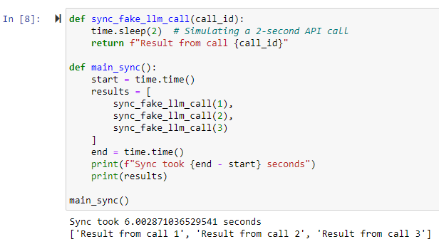
That’s three times slower! In a real-world application with multiple API calls, the difference can be even more dramatic.
Async Task Queue
When building LLM-powered applications with FastAPI, you’ll often encounter scenarios where you need to handle long-running tasks without blocking the main application (i.e. waiting for the LLM client to return data). This is where an async task queue comes in handy. It allows you to offload time-consuming operations (like complex LLM generations) to background workers, improving the responsiveness of your API.
Here’s a basic example of how you can implement an async task queue in FastAPI:
from fastapi import FastAPI, BackgroundTasks
from pydantic import BaseModel
import asyncio

app = FastAPI()

class Task(BaseModel):
    id: str
    status: str = "pending"
    result: str = None

tasks = {}

async def process_task(task_id: str):
    # Simulate a long-running LLM task
    await asyncio.sleep(10)
    tasks[task_id].status = "completed"
    tasks[task_id].result = f"Result for task {task_id}"

@app.post("/tasks")
async def create_task(background_tasks: BackgroundTasks):
    task_id = str(len(tasks) + 1)
    task = Task(id=task_id)
    tasks[task_id] = task
    background_tasks.add_task(process_task, task_id)
    return {"task_id": task_id}

@app.get("/tasks/{task_id}")
async def get_task(task_id: str):
    return tasks.get(task_id, {"error": "Task not found"})
In this example, we’re using FastAPI’s BackgroundTasks to manage our task queue. When a client creates a new task, we immediately return a task ID and start processing the task in the background. The client can then poll the /tasks/{task_id} endpoint to check the status of their task.
This approach has several advantages:
- Responsiveness: Your API can quickly acknowledge task creation without waiting for the task to complete.
- Scalability: You can easily distribute tasks across multiple workers.
- Fault Tolerance: If a task fails, it doesn’t bring down your entire application.
For more complex scenarios, you might want to consider using a dedicated task queue system like Celery or RQ (Redis Queue). These provide additional features like task prioritisation, retries, and distributed task processing. However, for many LLM applications, FastAPI’s built-in background tasks are more than sufficient.
(A few years ago I had to almost always resort to the more complex Celery or Redis, which came with it’s own set of headaches – async BackgroundTasks have come on a lot and are now easier and quicker to implement for most initial use cases.)
Here’s an example of running such a task queue in a Jupyter Notebook using a Test Client.

Remember, when working with async task queues, it’s crucial to handle errors gracefully and provide clear feedback to the client about the task’s status. You might also want to implement task timeouts and cleanup mechanisms to prevent your task queue from growing indefinitely.
Async LLM Clients
Both OpenAI and Anthropic now how working async clients. These were patchy or undocumented a few months ago but they are slowly gaining ground as part of the official documented software development kits (SDKs). The async clients allow you to make non-blocking API calls to LLM services. This can significantly improve the performance of applications that need to make multiple LLM requests concurrently.
OpenAI Async Client
OpenAI’s Python library supports async operations out of the box. Here’s a basic example of how to use it:
from openai import AsyncOpenAI
import asyncio

async def main():
    client = AsyncOpenAI()
    response = await client.chat.completions.create(
        model="gpt-4o",
        messages=[
            {"role": "system", "content": "You are a helpful assistant."},
            {"role": "user", "content": "What is the capital of France?"}
        ]
    )
    print(response.choices[0].message.content)

# This for in a script
asyncio.run(main())
# Or this for within Jupyter Notebooks
# For interactive environments (like Jupyter)
loop = asyncio.get_event_loop()
if loop.is_running():
    loop.create_task(main())
else:
    loop.run_until_complete(main())
Key points about OpenAI’s async client:
- It’s part of the official
openaiPython package. - You can create an
AsyncOpenAIclient to make async calls. - Most methods that make API requests have async versions.
- It’s compatible with Python’s
asyncioecosystem.
Anthropic Async Client
Anthropic also provides async support in their official Python library. Here’s a basic example:
from anthropic import AsyncAnthropic
import asyncio

async def main():
    client = AsyncAnthropic()
    response = await client.messages.create(
        model="claude-3-5-sonnet-20240620",
        max_tokens=300,
        messages=[
            {
                "role": "user",
                "content": "What is the capital of Spain?",
            }
        ],
    )
    print(response.content)

# This for in a script
asyncio.run(main())
# Or this for within Jupyter Notebooks
# For interactive environments (like Jupyter)
loop = asyncio.get_event_loop()
if loop.is_running():
    loop.create_task(main())
else:
    loop.run_until_complete(main())
Key points about Anthropic’s async client:
- It’s part of the official
anthropicPython package. - You can create an
AsyncAnthropicclient for async operations. - Most API methods have async counterparts.
- It integrates well with Python’s async ecosystem.
Benefits of Using Async Clients
- Improved Performance: You can make multiple API calls concurrently, reducing overall wait time.
- Better Resource Utilisation: Your application can do other work while waiting for API responses.
- Scalability: Async clients are better suited for handling high volumes of requests.
Async Libraries for Python
Python’s asyncio library is your bread and butter for async programming. However, you’ll also want to get familiar with libraries like aiohttp for making asynchronous HTTP requests, which you might need if interacting with other web-API services.
import aiohttp
import asyncio

async def fetch(session, url):
    async with session.get(url) as response:
        return await response.text()

async def main():
    async with aiohttp.ClientSession() as session:
        html = await fetch(session, 'http://python.org')
        print(html[:50])

# This for in a script
asyncio.run(main())
# Or this for within Jupyter Notebooks
# For interactive environments (like Jupyter)
loop = asyncio.get_event_loop()
if loop.is_running():
    loop.create_task(main())
else:
    loop.run_until_complete(main())
The Async Learning Curve
Now, I won’t lie to you – async programming can be a bit of a mind-bender at first. Concepts like coroutines, event loops, and futures might make you feel like you’re learning a whole new language. And in a way, you are. You’re learning to think about programming in a fundamentally different way.
The good news is that once it clicks, it clicks. And the performance benefits for LLM applications are well worth the initial struggle.
I’ve found support get a lot better over the last 12 months. Examples were pretty much non-existent a year ago. Now there are a few and LLMs are up to date enough to offer a first (non-working) example to get you going.
Testing and Debugging Async Code
One word of warning: testing and debugging async code can be… interesting. Race conditions and timing-dependent bugs can be tricky to reproduce and fix. Tools like pytest-asyncio can help, but be prepared for some head-scratching debugging sessions.
The Async Ecosystem is Still Maturing
As of 2024, the async ecosystem in Python is still a bit rough around the edges. Documentation can be sparse, and best practices are still evolving. But don’t let that deter you – async is the future for LLM applications, and the sooner you get on board, the better off you’ll be.
Remember, the goal here isn’t to make your code more complex. It’s to make your LLM applications more responsive and efficient. And in a world where every millisecond counts, that’s not just nice to have – it’s essential.
Parallelisation for High-Quality Output Generation
When it comes to LLM-powered applications, sometimes you need to go fast, and sometimes you need to go deep. Parallelisation lets you do both – if you’re clever about it.
Why Parallelise?
First off, let’s talk about why you’d want to parallelise your LLM requests:
- Speed: Obviously, doing things in parallel is faster than doing them sequentially. If you’re making multiple independent LLM calls, why wait for one to finish before starting the next?
- Improved Output Quality: By running multiple variations of a prompt in parallel, you can generate diverse outputs and then select or combine the best results.
- Handling Complex Tasks: Some tasks require multiple LLM calls with interdependent results. Parallelisation can help manage these complex workflows more efficiently.
Parallelisation Strategies
Here are a few strategies you can employ:
Simple Parallel Requests
This is the most straightforward approach. If you have multiple independent tasks, just fire them off concurrently.
import asyncio
from openai import AsyncOpenAI

async def generate_text(client, prompt):
    response = await client.chat.completions.create(
        model="gpt-4",
        messages=[{"role": "user", "content": prompt}]
    )
    return response.choices[0].message.content

async def main():
    client = AsyncOpenAI()
    prompts = [
        "Write a short poem about Python",
        "Explain quantum computing in simple terms",
        "List 5 benefits of exercise"
    ]
    results = await asyncio.gather(*(generate_text(client, prompt) for prompt in prompts))
    for prompt, result in zip(prompts, results):
        print(f"Prompt: {prompt}\nResult: {result}\n")

# This for in a script
asyncio.run(main())
# Or this for within Jupyter Notebooks
# For interactive environments (like Jupyter)
loop = asyncio.get_event_loop()
if loop.is_running():
    loop.create_task(main())
else:
    loop.run_until_complete(main())

Parallel Variations for Quality
Generate multiple variations of the same prompt in parallel, then select or combine the best results.
async def generate_variations(client, base_prompt, num_variations=3):
    tasks = []
    for i in range(num_variations):
        prompt = f"{base_prompt}\nVariation {i+1}:"
        tasks.append(generate_text(client, prompt))
    return await asyncio.gather(*tasks)

async def main():
    client = AsyncOpenAI()
    base_prompt = "Generate a catchy slogan for a new smartphone"
    variations = await generate_variations(client, base_prompt)
    print("Generated slogans:")
    for i, slogan in enumerate(variations, 1):
        print(f"{i}. {slogan.strip()}")

# This for in a script
asyncio.run(main())
# Or this for within Jupyter Notebooks
# For interactive environments (like Jupyter)
loop = asyncio.get_event_loop()
if loop.is_running():
    loop.create_task(main())
else:
    loop.run_until_complete(main())

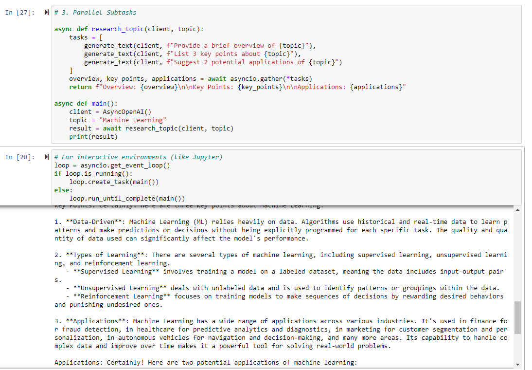
Parallel Subtasks
For complex tasks, break them down into subtasks that can be executed in parallel.
async def research_topic(client, topic):
    tasks = [
        generate_text(client, f"Provide a brief overview of {topic}"),
        generate_text(client, f"List 3 key points about {topic}"),
        generate_text(client, f"Suggest 2 potential applications of {topic}")
    ]
    overview, key_points, applications = await asyncio.gather(*tasks)
    return f"Overview: {overview}\n\nKey Points: {key_points}\n\nApplications: {applications}"

async def main():
    client = AsyncOpenAI()
    topic = "Machine Learning"
    result = await research_topic(client, topic)
    print(result)

# This for in a script
asyncio.run(main())
# Or this for within Jupyter Notebooks
# For interactive environments (like Jupyter)
loop = asyncio.get_event_loop()
if loop.is_running():
    loop.create_task(main())
else:
    loop.run_until_complete(main())
Considerations and Caveats
While parallelisation can significantly boost your application’s performance, it’s not without its challenges:
- API Rate Limits: Most LLM providers have rate limits. Make sure your parallel requests don’t exceed these limits, or you’ll end up with errors instead of speed gains. When working with legal applications my number of “matters” are normally in the thousands and my rate limits are in the order of millions per minute, so it makes sense to speed things up by running requests in parallel.
- Cost Considerations: Remember, each parallel request costs money. Make sure the benefits outweigh the increased API usage costs.
- Result Consistency: When generating variations, you might get inconsistent results. You’ll need a strategy to reconcile or choose between different outputs.
- Complexity: Parallel code can be harder to debug and maintain. Make sure the performance gains justify the added complexity.
- Resource Management: Parallelisation can be resource-intensive. Monitor your application’s memory and CPU usage, especially if you’re running on constrained environments.
Implementing Parallelisation
In Python, the asyncio library is your friend for implementing parallelisation. For more complex scenarios, you might want to look into libraries like aiohttp for making async HTTP requests, or even consider distributed task queues like Celery for large-scale parallelisation.
Remember, parallelisation isn’t a magic bullet. It’s a powerful tool when used judiciously, but it requires careful thought and implementation. Start simple, measure your gains, and scale up as needed. And always, always test thoroughly – parallel bugs can be particularly sneaky!
Leveraging LLMs in the Development Process
As developers, we’re always on the lookout for tools that can streamline our workflow and boost productivity. LLMs like ChatGPT and Claude have emerged as powerful allies in the development process. Let’s dive into how you can effectively leverage these AI assistants in your coding projects.
Setting Up Your LLM Workspace
One approach that’s worked well is setting up a dedicated Claude Project for each coding project. Here’s how you can structure this:
- Initialise the Project: Create a new Claude Project for your coding project (basically ~ to a GitHub repository).
- Load Key Materials: Populate the project with essential documents:
- Style guides and quality guidelines
- Project background and requirements
- Key code files developed so far
- Examples of similar implementations you admire
- Branch Management: Develop individual features on separate git branches, each with its own chat off the main project.
- Keep It Updated: As you progress, regularly update the project materials with the latest code files.
Leveraging LLMs for Feature Development
LLMs like Claude excel at quickly coding discrete features across 2-3 files, but they can struggle with integrating into complex existing systems. Here’s a strategy to make the most of their capabilities:
- Generate a Toy Version: Use Claude to create a standalone version of your feature.
- Implement as a Separate Package: Take the LLM-generated code and implement it on a new feature git branch as a separate Python package (i.e., folder) within the existing code repo.
- Iterate with Tests: Get the feature working independently, using tests to guide your iterations. Pop your tests in a separate test folder corresponding to your separate Python package.
- Manual Integration: Once your feature is working as desired, handle the integration into your main codebase yourself.
If you need to edit existing functions and classes:
- Find and Isolate Files and Tests: Identify the files that will be modified by your proposed update. This is generally the first step in bug fixing anyway. If in doubt, create a test that calls the method, function, or class you need to modify/fix/improve, then trace the call stack in an IDE debug mode (I use Pycharm Pro). Copy this files into the chat. Try to keep these below 3-5 (good coding practice anyway).
- Use Test-Driven Development: Write new tests in your existing suite that match the new functionality you want to implement.
- Get LLM to Sketch and Summarise the Existing Interfaces: Define your updates schematically first – set out new method interfaces, variables, and passed data. Use these in your tests (which should be failing at this stage).
- Fix the Interfaces and Generate Internal Code: Then get the LLM to fill in the functional code. Copy into your git branch and run the tests. Iterate pasting back the errors until you get something working.
- Aim for 100% Coverage and Use to Prevent Unintended Consequences: By generating tests as you code, you can ensure that other portions of you codes are covered by tests. This helps when you modify anything (LLMs and you will get it wrong first 1-3 times) – run the tests, see what is broke, work out why, fix, repeat until everything passes.
- Use Git/GitHub Pull Requests and Code Review: This is an extra review stage to catch dodgy LLM solutions that still pass the tests before integrating into your production code.
Best Practices and Considerations
While LLMs can be incredibly helpful, it’s important to use them judiciously:
- Code Review: Always review LLM-generated code thoroughly. These models can produce impressive results, but they can also make mistakes or introduce subtle bugs.
- Avoid Integration Hallucinations: LLMs like Claude or Copilot may hallucinate existing code structures. Don’t rely on them for integrating with your existing codebase.
- Use for Ideation: LLMs are excellent for brainstorming and getting quick prototypes. Use them to explore different approaches to a problem. I’m not a front-end person but in a few hours you can get a working React prototype you can show to frontend developers and go – something like this!
- Documentation and Comments: Ask the LLM to provide detailed comments and documentation for the code it generates. This can save you time and ensure better code understanding.
- Learning Tool: Use LLMs to explain complex code or concepts. They can be excellent teachers for new programming paradigms or libraries.
Real-World Example: Developing a New API Endpoint
Let’s say you’re adding a new API endpoint to your FastAPI application. Here’s how you might use Claude:
- Outline the Feature: Describe the new endpoint to Claude, including expected inputs and outputs.
- Generate Initial Code: Ask Claude to create a basic implementation, including the endpoint function, any necessary data models, and unit tests.
- Iterate and Refine: Use Claude to help refine the code, optimize performance, and enhance error handling.
- Documentation: Have Claude generate OpenAPI documentation for your new endpoint.
- Testing: Use Claude to suggest additional test cases and help implement them.
- Manual Integration: Once you’re satisfied with the standalone implementation, integrate it into your main application yourself.
The Limits of LLM Assistance
While LLMs are powerful tools, they’re not a replacement for human developers. They excel at certain tasks:
- Quick prototyping
- Explaining complex concepts
- Generating boilerplate code
- Suggesting optimisation techniques
But they struggle with:
- Understanding the full context of large codebases
- Making architectural decisions that affect the entire system
- Ensuring code aligns with all business rules and requirements
Integrating LLMs like Claude into your development process can significantly boost productivity and spark creativity. However, you need to understand their strengths and limitations. Use them as powerful assistants, but remember that the final responsibility for the code and its integration lies with you, the developer.
By leveraging LLMs thoughtfully in your workflow, you can accelerate feature development, improve code quality, and free up more of your time for the complex problem-solving that human developers do best.
Prompt Tips
Best practice on using prompts has been developing at a steady pace. The cycle seems to be:
- fudge something to get it working and get around limitations;
- have major LLM providers improve the limitations so the fudge isn’t needed as much;
- find documented examples where someone has had a better idea;
- GOTO 1.
Here are some aspects of using prompts that work at the moment.
Keep it Simple
Keep prompts simple.
Initially, I’d have lots of fancy string concatenation methods to generate conditional strings based on the content of my data. While this is helpful in streamlining the prompts and leaving out extra information that can sometimes confuse the LLM, it does make it difficult to view and evaluate prompts.
A better approach is to treat each LLM interaction as a single action with a single prompt. The single prompt has variable slots and these are populated by your logic code prior to the request.
Storage
A nice tool to use is Jinja templates. Those familiar with Flask will be well acquainted with these for creating HTML templates. But they can also be used for generating just text templates. And they have a long history of use and examples to help you.
Based on traditional Jinja template use, a good setup is to have a “prompt” or “prompt template” folder that has a number of text files (simple “.txt”).
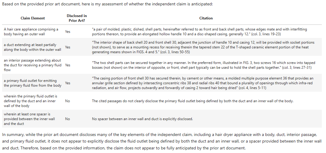
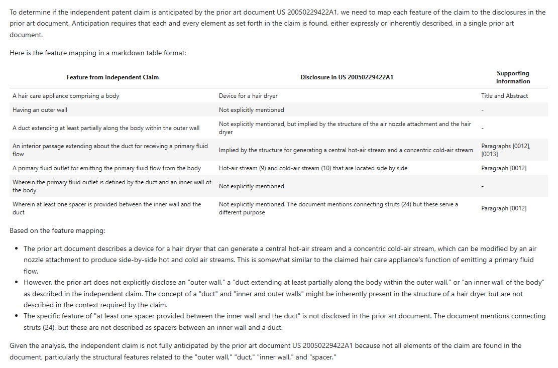
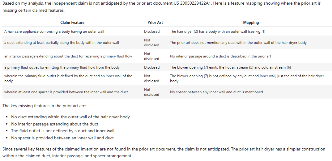
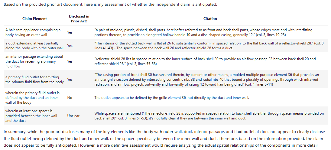
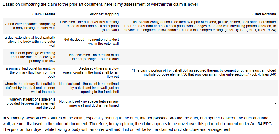
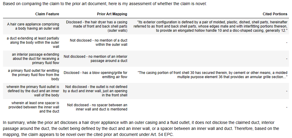
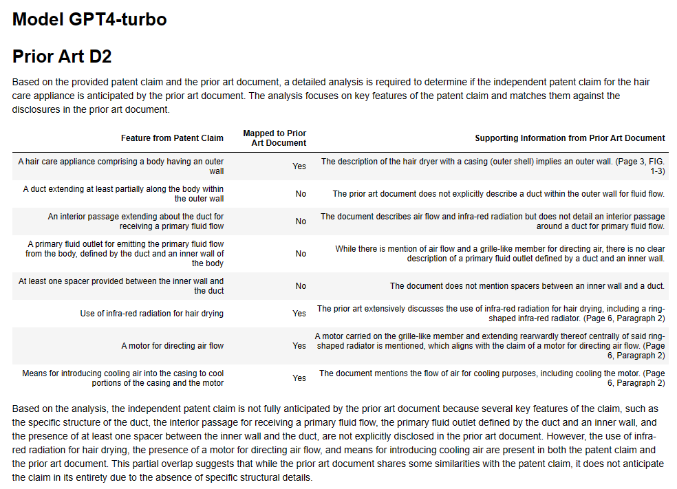
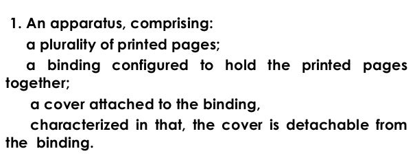
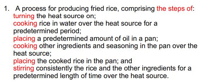
# prompt_templates/patent_review.txt
You are a patent analysis assistant.

Patent Document:
Title: {{ patent_title }}
Filing Date: {{ filing_date }}
Inventors: {{ inventors }}
Technology Field: {{ tech_field }}

Please analyse the following patent content:
---
{{ patent_content }}
---

Focus your analysis on:
1. Novel features claimed
2. Scope of protection
3. Potential prior art considerations
4. Commercial implications
# prompt_templates/contract_summary.txt
You are a contract analysis assistant.

Contract Details:
Title: {{ contract_title }}
Parties: {{ parties }}
Date: {{ contract_date }}
Type: {{ contract_type }}

Please analyse the following contract:
---
{{ contract_content }}
---

Provide a summary covering:
1. Key terms and conditions
2. Obligations of each party
3. Important deadlines
4. Risk areas
5. Recommended amendments
# prompt_templates/legal_analysis.txt
You are a legal assistant helping analyse documents.

Document Information:
Title: {{ document_title }}
Type: {{ document_type }}
Author: {{ author }}
Date Created: {{ date_created }}
Jurisdiction: {{ jurisdiction }}
Reviewer: {{ reviewer_name }}

Please analyse the following document content for {{ analysis_type }}:
---
{{ document_content }}
---

Provide a detailed analysis covering:
1. Key legal points
2. Potential issues or risks
3. Recommended actions
Here’s a short Python example that uses these:
# Directory structure:
# my_project/
# ├── prompt_templates/
# │   ├── legal_analysis.txt
# │   ├── patent_review.txt
# │   └── contract_summary.txt
# ├── db_connector.py
# └── prompt_manager.py

# db_connector.py
import sqlite3
from dataclasses import dataclass
from typing import Optional

@dataclass
class Document:
    id: int
    title: str
    content: str
    doc_type: str
    date_created: str
    author: Optional[str]

class DatabaseConnector:
    def __init__(self, db_path: str):
        self.db_path = db_path

    def get_document(self, doc_id: int) -> Document:
        with sqlite3.connect(self.db_path) as conn:
            cursor = conn.cursor()
            cursor.execute("""
                SELECT id, title, content, doc_type, date_created, author
                FROM documents
                WHERE id = ?
            """, (doc_id,))
            row = cursor.fetchone()

            if not row:
                raise ValueError(f"Document with id {doc_id} not found")

            return Document(
                id=row[0],
                title=row[1],
                content=row[2],
                doc_type=row[3],
                date_created=row[4],
                author=row[5]
            )

# prompt_manager.py
import os
from pathlib import Path
from typing import Dict, Any
from jinja2 import Environment, FileSystemLoader
from anthropic import Anthropic

class PromptManager:
    def __init__(self, templates_dir: str, anthropic_api_key: str):
        self.env = Environment(
            loader=FileSystemLoader(templates_dir),
            trim_blocks=True,
            lstrip_blocks=True
        )
        self.client = Anthropic(api_key=anthropic_api_key)

    def load_template(self, template_name: str) -> str:
        """Load a template file and return it as a string."""
        return self.env.get_template(f"{template_name}.txt")

    def render_prompt(self, template_name: str, variables: Dict[str, Any]) -> str:
        """Render a template with the provided variables."""
        template = self.load_template(template_name)
        return template.render(**variables)

    async def send_prompt(self, prompt: str, model: str = "claude-3-sonnet-20240229") -> str:
        """Send the rendered prompt to Claude and return the response."""
        message = await self.client.messages.create(
            model=model,
            max_tokens=4000,
            messages=[{"role": "user", "content": prompt}]
        )
        return message.content

# Example usage
async def main():
    # Initialize managers
    db = DatabaseConnector("legal_docs.db")
    prompt_mgr = PromptManager(
        templates_dir="prompt_templates",
        anthropic_api_key="your-api-key"
    )

    # Get document from database
    doc = db.get_document(doc_id=123)

    # Prepare variables for template
    variables = {
        "document_title": doc.title,
        "document_content": doc.content,
        "document_type": doc.doc_type,
        "author": doc.author or "Unknown",
        "date_created": doc.date_created,
        "analysis_type": "legal_review",
        "jurisdiction": "UK",
        "reviewer_name": "John Smith"
    }

    # Render prompt from template
    prompt = prompt_mgr.render_prompt("legal_analysis", variables)

    # Send to Claude and get response
    response = await prompt_mgr.send_prompt(prompt)
    print(response)

if __name__ == "__main__":
    import asyncio
    asyncio.run(main())
Versioning
You’ll endlessly tweak your prompts. This makes it difficult to keep on track of changes.
Git is your first friend here. Make sure your template directory is added to git, so you can track changes over time. If you host your code in GitHub or GitBucket you can use a web-interface to flick through different versions of the prompts with different commits.
You might also want to set up a manual or automated version numbering system (e.g. 0.1.0, 2.2.12) to reflect changes as you go along. This could be available programmatically and stored with your prompt in logs and test examples.
Make it Easy to Test
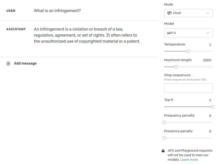
The Anthropic Workbench has got a lot better over the last year and provides a template for how to structure prompts.
The Workbench has a “Prompt” screen where you can compose and test prompts and an “Evaluate” screen where you can evaluate prompts over a number of runs. The Evaluate option provides a useful guide to how you can evaluate prompts over time.
Build a Test Dataset
Use a machine-learning style dataset with input and output pairs, where the output is a ground-truth example. Structure your input as per your prompt variables. Anthropic Workbench allows you to upload examples in CSV format. So think about storing this data in a spreadsheet style format (you can always stored in a database and write a script to convert to CSV via pandas).
Each row of your test dataset should have column headings that reflect your prompt variables, then a column that represents an “ideal_output”, then a column “model_output” that can be used to store results. The Workbench also uses a scoring system so you might want to add a “score” column for recording a manually assigned score from 1 (Poor) to 5 (Excellent).
Data arranged in this way can then be uploaded and exported from the Anthropic Workbench, allowing you to quickly compare Anthropic models.
I’d also recommend storing the current version of your prompt, either by copying and pasting or (better) providing a link to the current prompt file and current version (e.g., GitHub link and commit hash).
If your data is arranged in this format you can also write little scripts to automate sending the examples off into APIs and record the results.
Prompt Logging
API calls cost money. But you often need to run end-to-end tests through the LLM API. It can also be difficult to debug LLM applications – is the problem in your code and logic or in the prompt?
Proper logging of prompts can help you trace errors and find out exactly what you were sending to the LLM. Problem is prompts are often long and verbose. Simple standard output line logging falls down and other logging gets drowned out by logged API calls and responses.
Another problem is the actual LLM call can have a series of text and/or image user messages, but a human needs to read the simple flattened LLM text with populated data. Also images are transmitted as base64 encoded strings – you need to filter these out of your prompts otherwise they will take over any logs with encoded string rubbish.
There are several companies out there that propose to sell LLM logging solutions. But I find them complex and they often involve sending yet more data off into a nondescript third party cloud – not great if you are trying to secure the call chain.
If I was clever, I’d be able to set up a separate Python logger for the LLM calls and have this log to a separate database.
But I’m not. So as a compromise, I’ve found that a simple standalone JSON or MongoDB package I can reuse across projects works well. I can then pass the messages that I pass to the LLM client, and write some simple code to flatten this and save it as a cleaned string. I can then save with some UUIDs of related objects/users/tasks to then trace it back to a code flow.
Conclusion
As we’ve explored in this post covering technical implementations of LLM-powered systems, building robust applications requires careful consideration of architecture, asynchronous programming, parallelisation strategies, and thoughtful prompt engineering. The rapid evolution of LLM capabilities means we’re often building tomorrow’s solutions with today’s tools, requiring flexibility and adaptability in our approach.
We’ve seen how a well-structured tech stack, centered around FastAPI and modern async programming patterns, can provide a solid foundation for LLM applications. The move towards asynchronous programming isn’t just a performance optimisation—it’s becoming essential for handling the inherently slow nature of LLM API calls effectively. Similarly, parallelisation strategies offer powerful ways to improve both speed and output quality, though they require careful management of resources and rate limits.
The integration of LLMs into the development process itself represents an interesting meta-level application of these technologies. While they can significantly accelerate certain aspects of development, success lies in understanding their limitations and using them judiciously as part of a broader development strategy.
Perhaps most importantly, we’ve learned that effective implementation isn’t just about the code—it’s about creating sustainable, maintainable systems. This means paying attention to prompt management, testing strategies, and logging systems that can help us understand and improve our LLM applications over time.
In our next and final post in this series, we’ll examine the persistent challenges and issues that remain in working with LLMs, including questions of reliability, evaluation, and the limitations we continue to encounter. Until then, remember that we’re all still pioneers in this rapidly evolving field—don’t be afraid to experiment, but always build with care and consideration for the future.